Understanding the Buffon-Laplace Needle Problem
This page explains the probability model behind the interactive demo and shows how repeated random trials can be used to estimate .
1. The Classic Starting Point: Buffon's Needle
In 1733, the French naturalist Georges-Louis Leclerc, Comte de Buffon posed a deceptively simple question:
If a needle of length is dropped randomly onto a floor ruled with parallel lines spaced apart (where ), what is the probability that the needle crosses a line?
The answer turns out to be:
This result is remarkable because a physical random experiment gives a way to estimate . The more times the needle is dropped, the better the estimate becomes.
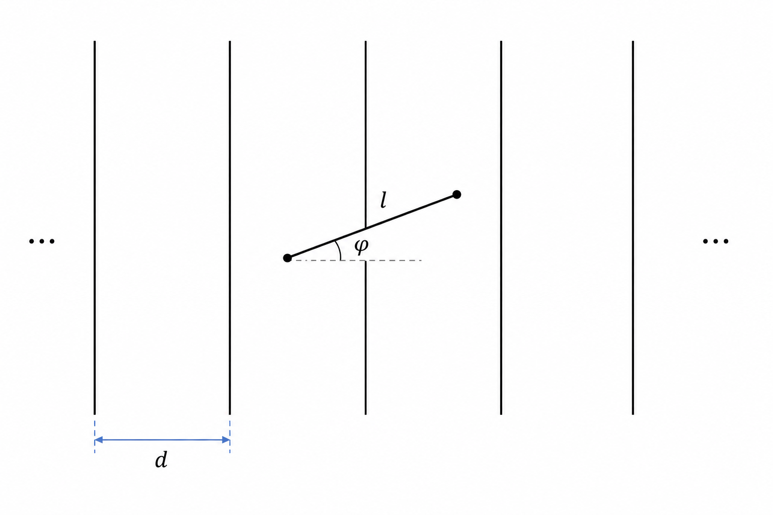
But if there are lines on the floor both horizontally and vertically, what interesting things would that be?
2. Extending to Two Dimensions: The Buffon-Laplace Problem
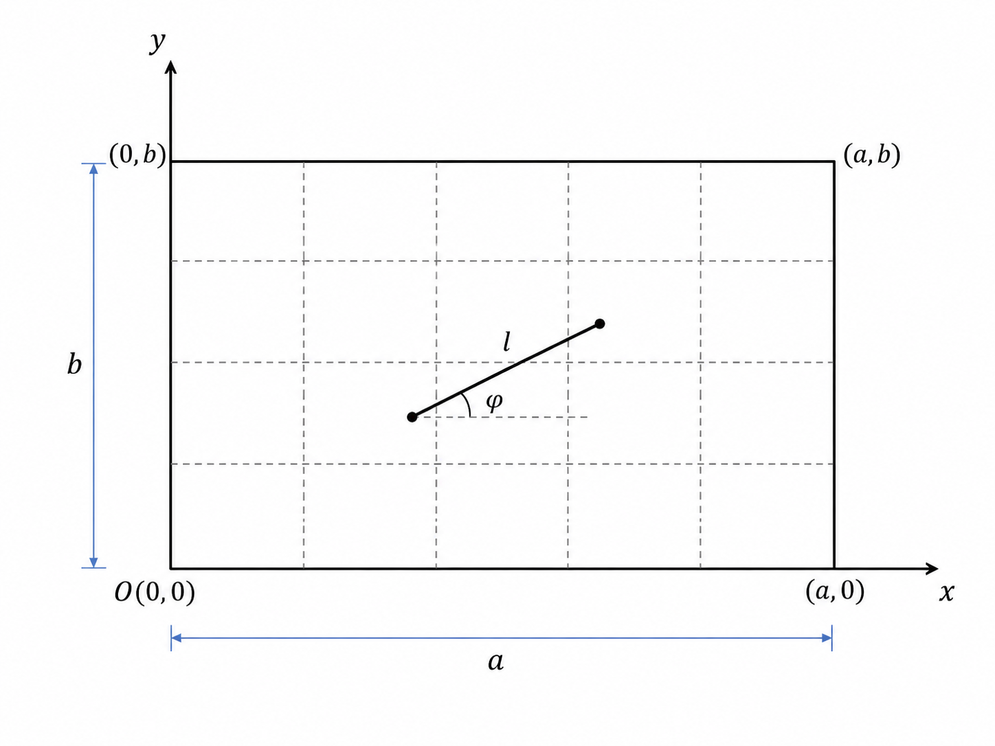
The Buffon-Laplace Needle Problem generalises the original version by replacing the parallel lines with a rectangular grid: horizontal lines spaced apart and vertical lines spaced apart.
A needle of length (with and ) is dropped randomly. We now ask: what is the probability that the needle crosses at least one grid line?
This version was first attempted by Buffon in 1777, but his derivation contained an error. A correct solution was later published by Pierre-Simon Laplace in 1812, which is why the problem carries both names.
3. Setting Up the Model
3.1 Modeling Assumptions
To formalise the problem rigorously, we make the following assumptions:
- Periodicity of the grid: The rectangular grid can be treated as a repeating tiling of identical cells, so it is enough to analyse the needle within one cell.
- Uniform distribution of the centre: The centre point of the needle is uniformly distributed over the rectangle:
- Independence of position and orientation: The orientation of the needle is independent of its position .
- Uniform distribution of orientation: Due to rotational symmetry, the angle satisfies:
These assumptions define a uniform probability distribution over the sample space:
The probability of any event is then the ratio of the corresponding volume in to the total volume , which justifies the integration approach used in the derivation.
3.2 Crossing Conditions
The needle's state is fully described by the three random variables above. Using them, we can express when the needle reaches a grid line.
The needle crosses a vertical line when its horizontal projection reaches a line:
The needle crosses a horizontal line when its vertical projection reaches a line:
4. Deriving the Probability
It is easier to first compute the probability that the needle crosses no lines, meaning the centre stays far enough from all four sides of the cell. At a fixed angle , this safe area is:
The last term corrects for the overlap where the needle is close to both a horizontal line and a vertical line at the same time.
Integrating over all angles and dividing by the total volume gives:
Evaluating this integral and subtracting from 1 yields the closed-form result:
5. Estimating
Rearranging the formula above lets us solve for :
In a simulation with needle drops, if of them result in a crossing, we estimate , giving:
By the Law of Large Numbers, as
,
converges to the true value of
.
i.e.,
6. What to Learn from the Demo
- More throws mean a better estimate: watch stabilise as increases.
- The effect of needle length: a longer needle crosses lines more often, which changes the estimated hit probability.
- The effect of grid spacing: larger values of and reduce the chance of a crossing.